Turning Lanes and Rsyslog Queues
If there is a single object absolutely vital to understanding the way rsyslog works, this object is queues. Queues offer a variety of services, including support for multithreading. While there is elaborate in-depth documentation on the ins and outs of rsyslog queues, some of the concepts are hard to grasp even for experienced people. I think this is because rsyslog uses a very high layer of abstraction which includes things that look quite unnatural, like queues that do not actually queue…
With this document, I take a different approach: I will not describe every specific detail of queue operation but hope to be able to provide the core idea of how queues are used in rsyslog by using an analogy. I will compare the rsyslog data flow with real-life traffic flowing at an intersection.
But first let’s set the stage for the rsyslog part. The graphic below describes the data flow inside rsyslog:
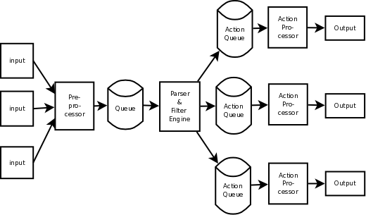
rsyslog data flow
Note that there is a video tutorial available on the data flow. It is not perfect, but may aid in understanding this picture.
For our needs, the important fact to know is that messages enter rsyslog on “the left side” (for example, via UDP), are preprocessed, put into the so-called main queue, taken off that queue, filtered and are placed into one or several action queues (depending on filter results). They leave rsyslog on “the right side” where output modules (like the file or database writer) consume them.
So there are always two stages where a message (conceptually) is queued - first in the main queue and later on in n action specific queues (with n being the number of actions that the message in question needs to be processed by, what is being decided by the “Filter Engine”). As such, a message will be in at least two queues during its lifetime (with the exception of messages being discarded by the queue itself, but for the purpose of this document, we will ignore that possibility).
Also, it is vitally important to understand that each action has a queue sitting in front of it. If you have dug into the details of rsyslog configuration, you have probably seen that a queue mode can be set for each action. And the default queue mode is the so-called “direct mode”, in which “the queue does not actually enqueue data”. That sounds silly, but is not. It is an important abstraction that helps keep the code clean.
To understand this, we first need to look at who is the active component. In our data flow, the active part always sits to the left of the object. For example, the “Preprocessor” is being called by the inputs and calls itself into the main message queue. That is, the queue receiver is called, it is passive. One might think that the “Parser & Filter Engine” is an active component that actively pulls messages from the queue. This is wrong! Actually, it is the queue that has a pool of worker threads, and these workers pull data from the queue and then call the passively waiting Parser and Filter Engine with those messages. So the main message queue is the active part, the Parser and Filter Engine is passive.
Let’s now try an analogy for this part: Think about a TV show. The show is produced in some TV studio, from there sent (actively) to a radio tower. The radio tower passively receives from the studio and then actively sends out a signal, which is passively received by your TV set. In our simplified view, we have the following picture:
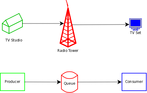
rsyslog queues and TV analogy
The lower part of the picture lists the equivalent rsyslog entities, in an abstracted way. Every queue has a producer (in the above sample the input) and a consumer (in the above sample the Parser and Filter Engine). Their active and passive functions are equivalent to the TV entities that are listed on top of the rsyslog entity. For example, a rsyslog consumer can never actively initiate reception of a message in the same way a TV set cannot actively “initiate” a TV show - both can only “handle” (display or process) what is sent to them.
Now let’s look at the action queues: here, the active part, the producer, is the Parser and Filter Engine. The passive part is the Action Processor. The latter does any processing that is necessary to call the output plugin, in particular it processes the template to create the plugin calling parameters (either a string or vector of arguments). From the action queue’s point of view, Action Processor and Output form a single entity. Again, the TV set analogy holds. The Output does not actively ask the queue for data, but rather passively waits until the queue itself pushes some data to it.
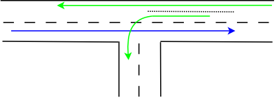
Armed with this knowledge, we can now look at the way action queue modes work. My analogy here is a junction, as shown below (note that the colors in the pictures below are not related to the colors in the pictures above!):
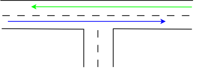
This is a very simple real-life traffic case: one road joins another. We look at traffic on the straight road, here shown by blue and green arrows. Traffic in the opposing direction is shown in blue. Traffic flows without any delays as long as nobody takes turns. To be more precise, if the opposing traffic takes a (right) turn, traffic still continues to flow without delay. However, if a car in the red traffic flow intends to do a (left, then) turn, the situation changes:
The turning car is represented by the green arrow. It cannot turn unless there is a gap in the “blue traffic stream”. And as this car blocks the roadway, the remaining traffic (now shown in red, which should indicate the block condition), must wait until the “green” car has made its turn. So a queue will build up on that lane, waiting for the turn to be completed. Note that in the examples below I do not care that much about the properties of the opposing traffic. That is, because its structure is not really important for what I intend to show. Think about the blue arrow as being a traffic stream that most of the time blocks left-turners, but from time to time has a gap that is sufficiently large for a left-turn to complete.
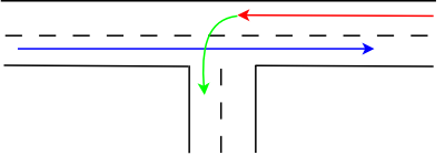
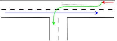
Our road network designers know that this may be unfortunate, and for more important roads and junctions, they came up with the concept of turning lanes:
Now, the car taking the turn can wait in a special area, the turning lane. As such, the “straight” traffic is no longer blocked and can flow in parallel to the turning lane (indicated by a now-green-again arrow).
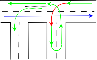
However, the turning lane offers only finite space. So if too many cars intend to take a left turn, and there is no gap in the “blue” traffic, we end up with this well-known situation:
The turning lane is now filled up, resulting in a tailback of cars intending to left turn on the main driving lane. The end result is that “straight” traffic is again being blocked, just as in our initial problem case without the turning lane. In essence, the turning lane has provided some relief, but only for a limited amount of cars. Street system designers now try to weight cost vs. benefit and create (costly) turning lanes that are sufficiently large to prevent traffic jams in most, but not all cases.
Now let’s dig a bit into the mathematical properties of turning lanes. We assume that cars all have the same length. So, units of cars, the length is always one (which is nice, as we don’t need to care about that factor any longer ;)). A turning lane has finite capacity of n cars. As long as the number of cars wanting to take a turn is less than or equal to n, “straight traffic” is not blocked (or the other way round, traffic is blocked if at least n + 1 cars want to take a turn!). We can now find an optimal value for n: it is a function of the probability that a car wants to turn and the cost of the turning lane (as well as the probability there is a gap in the “blue” traffic, but we ignore this in our simple sample). If we start from some finite upper bound of n, we can decrease n to a point where it reaches zero. But let’s first look at n = 1, in which case exactly one car can wait on the turning lane. More than one car, and the rest of the traffic is blocked. Our everyday logic indicates that this is actually the lowest boundary for n.
In an abstract view, however, n can be zero and that works nicely. There still can be n cars at any given time on the turning lane, it just happens that this means there can be no car at all on it. And, as usual, if we have at least n + 1 cars wanting to turn, the main traffic flow is blocked. True, but n + 1 = 0 + 1 = 1 so as soon as there is any car wanting to take a turn, the main traffic flow is blocked (remember, in all cases, I assume no sufficiently large gaps in the opposing traffic).
This is the situation our everyday perception calls “road without turning lane”. In my math model, it is a “road with turning lane of size 0”. The subtle difference is important: my math model guarantees that, in an abstract sense, there always is a turning lane, it may just be too short. But it exists, even though we don’t see it. And now I can claim that even in my small home village, all roads have turning lanes, which is rather impressive, isn’t it? ;)
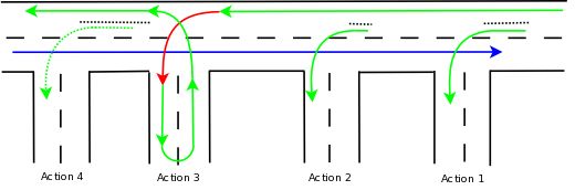
And now we finally have arrived at rsyslog’s queues! Rsyslog action queues exists for all actions just like all roads in my village have turning lanes! And as in this real-life sample, it may be hard to see the action queues for that reason. In rsyslog, the “direct” queue mode is the equivalent to the 0-sized turning lane. And actions queues are the equivalent to turning lanes in general, with our real-life n being the maximum queue size. The main traffic line (which sometimes is blocked) is the equivalent to the main message queue. And the periods without gaps in the opposing traffic are equivalent to execution time of an action. In a rough sketch, the rsyslog main and action queues look like in the following picture.

We need to read this picture from right to left (otherwise I would need to redo all the graphics ;)). In action 3, you see a 0-sized turning lane, aka an action queue in “direct” mode. All other queues are run in non-direct modes, but with different sizes greater than 0.
Let us first use our car analogy: Assume we are in a car on the main lane that wants to take turn into the “action 4” road. We pass action 1, where a number of cars wait in the turning lane and we pass action 2, which has a slightly smaller, but still not filled up turning lane. So we pass that without delay, too. Then we come to “action 3”, which has no turning lane. Unfortunately, the car in front of us wants to turn left into that road, so it blocks the main lane. So, this time we need to wait. An observer standing on the sidewalk may see that while we need to wait, there are still some cars in the “action 4” turning lane. As such, even though no new cars can arrive on the main lane, cars still turn into the “action 4” lane. In other words, an observer standing in “action 4” road is unable to see that traffic on the main lane is blocked.
Now on to rsyslog: Other than in the real-world traffic example, messages in rsyslog can - at more or less the same time - “take turns” into several roads at once. This is done by duplicating the message if the road has a non-zero-sized “turning lane” - or in rsyslog terms a queue that is running in any non-direct mode. If so, a deep copy of the message object is made, that placed into the action queue and then the initial message proceeds on the “main lane”. The action queue then pushes the duplicates through action processing. This is also the reason why a discard action inside a non-direct queue does not seem to have an effect. Actually, it discards the copy that was just created, but the original message object continues to flow.
In action 1, we have some entries in the action queue, as we have in action 2 (where the queue is slightly shorter). As we have seen, new messages pass action one and two almost instantaneously. However, when a messages reaches action 3, its flow is blocked. Now, message processing must wait for the action to complete. Processing flow in a direct mode queue is something like a U-turn:
message processing in an rsyslog action queue in direct mode
The message starts to execute the action and once this is done, processing flow continues. In a real-life analogy, this may be the route of a delivery man who needs to drop a parcel in a side street before he continues driving on the main route. As a side-note, think of what happens with the rest of the delivery route, at least for today, if the delivery truck has a serious accident in the side street. The rest of the parcels won’t be delivered today, will they? This is exactly how the discard action works. It drops the message object inside the action and thus the message will no longer be available for further delivery - but as I said, only if the discard is done in a direct mode queue (I am stressing this example because it often causes a lot of confusion).
Back to the overall scenario. We have seen that messages need to wait for action 3 to complete. Does this necessarily mean that at the same time no messages can be processed in action 4? Well, it depends. As in the real-life scenario, action 4 will continue to receive traffic as long as its action queue (“turn lane”) is not drained. In our drawing, it is not. So action 4 will be executed while messages still wait for action 3 to be completed.
Now look at the overall picture from a slightly different angle:
message processing in an rsyslog action queue in direct mode
The number of all connected green and red arrows is four - one each for action 1, 2 and 4 (this one is dotted as action 4 was a special case) and one for the “main lane” as well as action 3 (this one contains the sole red arrow). This number is the lower bound for the number of threads in rsyslog’s output system (“right-hand part” of the main message queue)! Each of the connected arrows is a continuous thread and each “turn lane” is a place where processing is forked onto a new thread. Also, note that in action 3 the processing is carried out on the main thread, but not in the non-direct queue modes.
I have said this is “the lower bound for the number of threads…”. This is with good reason: the main queue may have more than one worker thread (individual action queues currently do not support this, but could do in the future - there are good reasons for that, too but exploring why would finally take us away from what we intend to see). Note that you configure an upper bound for the number of main message queue worker threads. The actual number varies depending on a lot of operational variables, most importantly the number of messages inside the queue. The number t_m of actually running threads is within the integer-interval [0,confLimit] (with confLimit being the operator configured limit, which defaults to 5). Output plugins may have more than one thread created by themselves. It is quite unusual for an output plugin to create such threads and so I assume we do not have any of these. Then, the overall number of threads in rsyslog’s filtering and output system is t_total = t_m + number of actions in non-direct modes. Add the number of inputs configured to that and you have the total number of threads running in rsyslog at a given time (assuming again that inputs utilize only one thread per plugin, a not-so-safe assumption).
A quick side-note: I gave the lower bound for t_m as zero, which is somewhat in contrast to what I wrote at the beginning of the last paragraph. Zero is actually correct, because rsyslog stops all worker threads when there is no work to do. This is also true for the action queues. So the ultimate lower bound for a rsyslog output system without any work to carry out actually is zero. But this bound will never be reached when there is continuous flow of activity. And, if you are curious: if the number of workers is zero, the worker wakeup process is actually handled within the threading context of the “left-hand-side” (or producer) of the queue. After being started, the worker begins to play the active queue component again. All of this, of course, can be overridden with configuration directives.
When looking at the threading model, one can simply add n lanes to the main lane but otherwise retain the traffic analogy. This is a very good description of the actual process (think what this means to the “turning lanes”; hint: there still is only one per action!).
Let’s try to do a warp-up: I have hopefully been able to show that in rsyslog, an action queue “sits in front of” each output plugin. Messages are received and flow, from input to output, over various stages and two level of queues to the outputs. Actions queues are always present, but may not easily be visible when in direct mode (where no actual queuing takes place). The “road junction with turning lane” analogy well describes the way - and intent - of the various queue levels in rsyslog.
On the output side, the queue is the active component, not the consumer. As such, the consumer cannot ask the queue for anything (like n number of messages) but rather is activated by the queue itself. As such, a queue somewhat resembles a “living thing” whereas the outputs are just tools that this “living thing” uses.
Note that I left out a couple of subtleties, especially when it comes to error handling and terminating a queue (you hopefully have now at least a rough idea why I say “terminating a queue” and not “terminating an action” - who is the “living thing”?). An action returns a status to the queue, but it is the queue that ultimately decides which messages can finally be considered processed and which not. Please note that the queue may even cancel an output right in the middle of its action. This happens, if configured, if an output needs more than a configured maximum processing time and is a guard condition to prevent slow outputs from deferring a rsyslog restart for too long. Especially in this case re-queuing and cleanup is not trivial. Also, note that I did not discuss disk-assisted queue modes. The basic rules apply, but there are some additional constraints, especially in regard to the threading model. Transitioning between actual disk-assisted mode and pure-in-memory-mode (which is done automatically when needed) is also far from trivial and a real joy for an implementer to work on ;).
If you have not done so before, it may be worth reading Understanding rsyslog Queues, which most importantly lists all the knobs you can turn to tweak queue operation.
Conceptual model
rsyslog message flow mirrors traffic: the main queue drives processing and pushes work to passive consumers.
Every action conceptually has a queue; “direct” mode is equivalent to a zero-capacity turning lane that still gates flow.
Non-direct queues duplicate messages for parallel delivery, isolating slow actions from the main path.
Queue workers are the active agents pulling from queues and invoking parsers or actions; consumers never request data.
Queue capacity and worker counts bound concurrency: more lanes/queues increase parallelism, while zero-capacity queues serialize.
Shutdown, error handling, and timeouts are governed by the queue, which decides completion and can cancel long-running actions.
Support: rsyslog Assistant | GitHub Discussions | GitHub Issues: rsyslog source project
Contributing: Source & docs: rsyslog source project
© 2008–2025 Rainer Gerhards and others. Licensed under the Apache License 2.0.